Focused Ultrasound and MRI Physics

by Yoyo • 04-09-2026 #ultrasound #MRI

1. A fantastic stimulation at Lucas Center!

One sleepy morning, I appeared for a transcranial ultrasound study at the Lucas Centre at Stanford, where I was sent into an MRI machine, asked to focus on a visual stimulus and click buttons accordingly. Despite my sleepiness, the force is extremely strong with this one (metaphorical and literal), and I instantly focused!

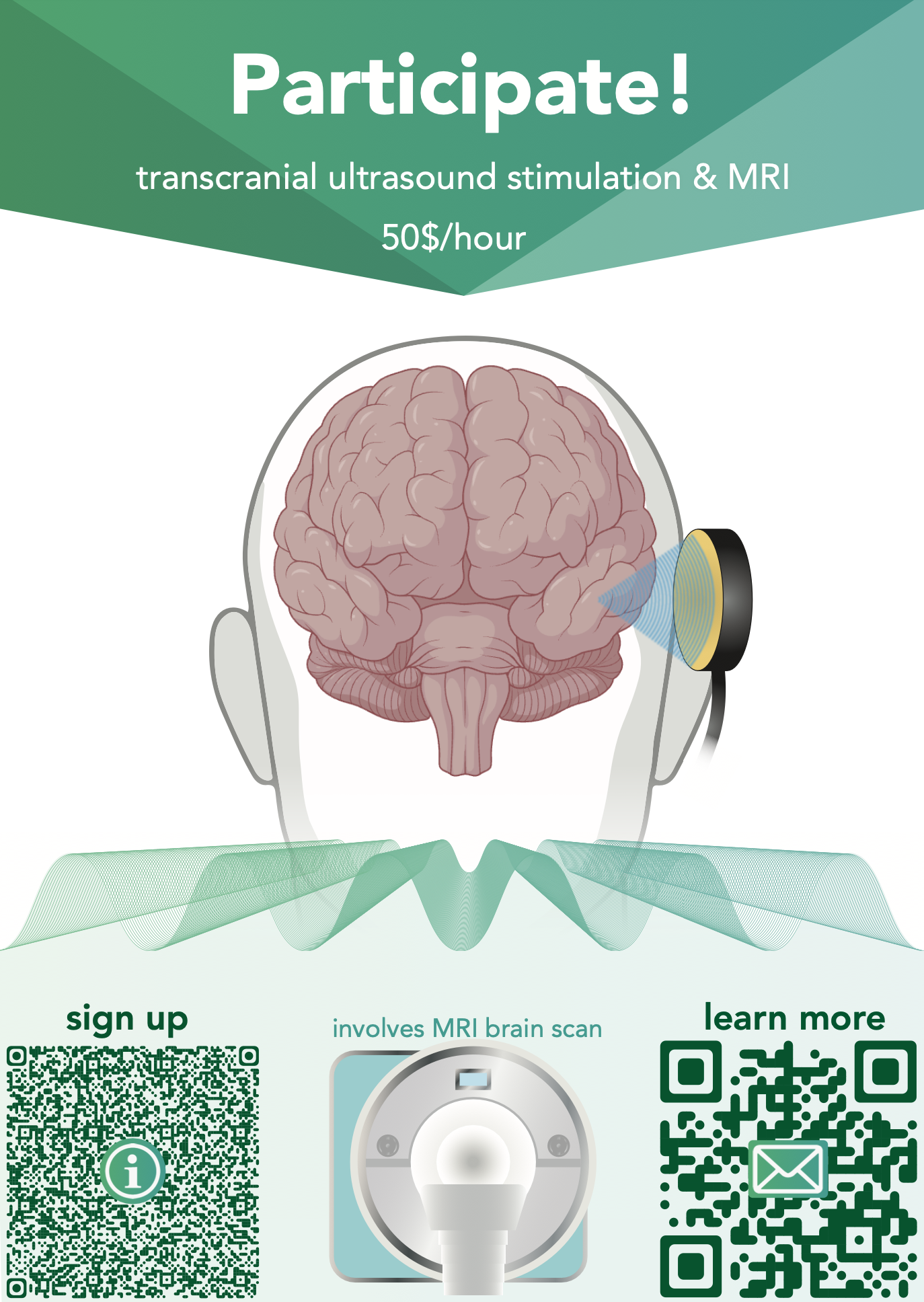
Fig 1. A flyer recruiting for a focused ultrasound study at Lucas Center.

Historically, MRI has dominated the medical imaging of the brain. Ultrasound was traditionally considered inadequate for neuroimaging, due to a series of reflection issues making the image blurry, but algorithmic improvements have caught up to speed these days to remain hopeful.

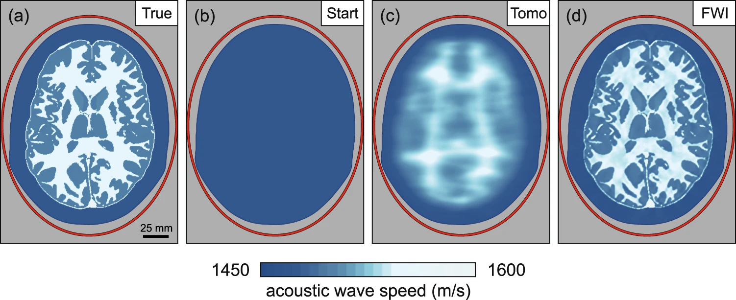
Fig 2. A resolution enhancement technique from Guasch et al. (2020), contrasting unimproved ultrasound (c) to improved FWI ultrasound (d). Source: Nature Digital Medicine [8].

2. MRI electromagnetism and ultrasound wave physics

Each of MRI and ultrasound exploits different tissue properties and wave physics. Ultrasound stimulates the brain via mechanical pressure waves and is favoured for its capabilities to reach deep structures with a handheld device at a reasonable cost. One simply applies conductive gel on the subject’s head and sets the transducer array on top. Then, pulses of ultrasound are delivered, transmitting via longitudinal pressure waves into the tissue.

Fig 3. An ultrasound transducer array on the subject’s head. Source: Deffieux et al. [6].

2.1 Acoustic Radiation Force

Newton’s second law, F = ma, is applied: momentum from the focused ultrasound wave is transferred into the tissue and then imaged. When this longitudinal pressure wave is absorbed or reflected by a medium, the momentum is transferred into a force known as the Acoustic Radiation Force (ARF), calculated as:

F = 2αP² / (ρ₀c²) = (2α / c) · I

where α is the absorption coefficient, P is the acoustic pressure, ρ₀ is the medium density, c is the speed of sound, and I is the acoustic intensity.

2.2 The Acoustic Wave Equation

In three dimensions, the acoustic wave equation is:

∇²p − (1/c²) · ∂²p/∂t² = 0

Here, ∇² is the Laplace operator (also called the Laplacian), which computes the sum of second partial derivatives across all spatial dimensions: ∇² = ∂²/∂x² + ∂²/∂y² + ∂²/∂z². It is a term describing local curvature of the pressure field. p is the local acoustic pressure, and c is the speed of sound. This PDE is derived from Newton’s second law applied to a continuous fluid element and the bulk modulus relation [1]

2.3 MRI basics

MRI is an imaging tool based on the water nuclei within the human body and their responses to magnetic fields. Initially, within the water nuclei, the protons are randomly oriented. A radio-frequency (RF) pulse, which is a burst of electromagnetic energy, disturbs the water nuclei. The nuclei have excess energy and will, after a certain period, spontaneously lose the energy by emitting another RF signal as they relax. These signals are measured by the computer [2].

During the time when protons have gained energy, they rotate about their axis, known as precession. The precession varies in frequency, known as the Larmor frequency:

f = γB

where γ is the Larmor constant (magnetogyric ratio) and B is the magnetic field strength. The Larmor frequency is sent back to the computer.

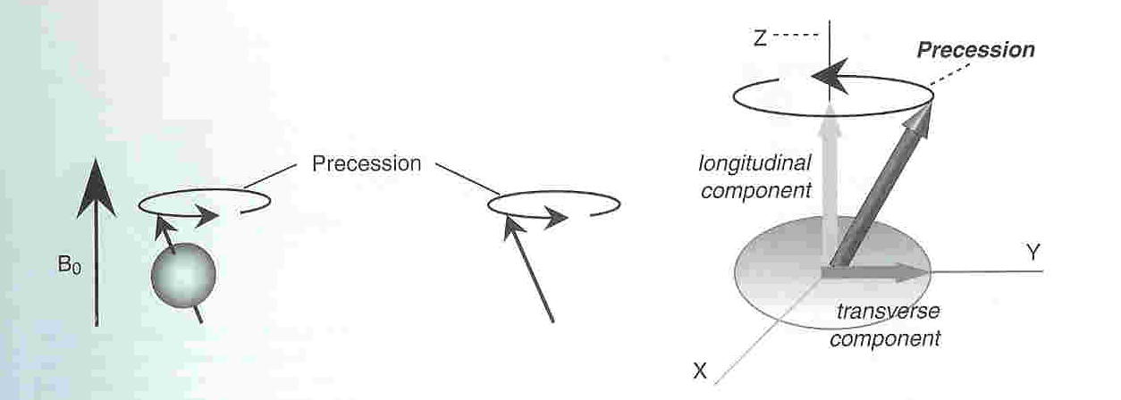
Fig 4. Diagram of a singular proton precessing. Source: UPenn MRI Basics [2].

How does the computer distinguish between multiple different protons with the same Larmor frequency? One answer is to produce different frequencies by varying the magnetic fields. Inside an MRI machine are three coils that coordinate to do this:

First, the main coil produces a uniform magnetic field for the scanner as a backdrop.

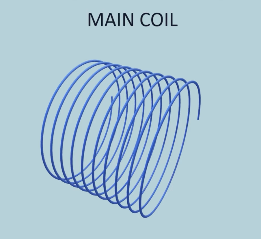
Fig 5. The main coil inside an MRI scanner. Source: MRI coils explanation [3].

Second, along the z-axis, several subcoils introduce a linear gradient of intensifying magnetic field. As the magnetic field becomes stronger, the Larmor frequency of protons also increases. Thus, the frequency becomes a function of position along the z-axis, also known as the technique of Motion Encoding Gradients (MEG).

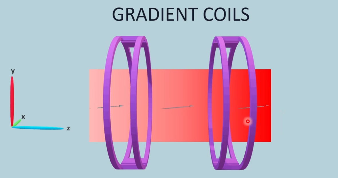
Fig 6. Gradient coils showing a linear gradient. Source: MRI coils explanation [3].

Finally, the RF coil delivers specific frequencies, perturbing only the protons whose natural precession frequency matches the RF. Each snapshot is a 2D picture which is stacked into a 3D structure of the brain.

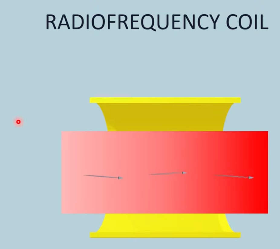
Fig 7. The RF coil inside MRI. Source: Source: MRI coils explanation [3].

3. MRI and ultrasound, one after the other

As the ultrasound stimulates, MRI watches the brain activity. However, the biological tissue behaves like an overdamped harmonic system: it shifts positions during ultrasound, and a bit after the sound turns off, relaxes back to the original spot. Simultaneously stimulating and recording with MRI is not actually the optimal approach. The displacement as a function of time can be modelled as:

D_rise(t) = (F/k)(1 − e^(−t/τ_rise))

D_fall(t) = D(T_off) · e^(−t/τ_fall)

K is a proportionality constant resembling the k in Hooke’s law, while τ_rise and τ_fall resemble the capacitor discharge constant. For brain tissue, the rise time is roughly 5.97 milliseconds with a shear wave speed of 1.56 m/s [4].

Brain tissue is heterogeneous in stiffness. (Side note: one modern challenge in neurotechnology is to match the stiffness of the brain with the implant so that it doesn’t get squished.) Young’s modulus provides a measure of strain [7]:

E = stress / strain = (F · L₀) / (A · ΔL)

If an area is destroyed by heat (a common scenario when ablating brain tumours with ultrasound) ΔL decreases, effectively increasing overall stiffness.

Considering the delayed movement of protons in the magnetic field in response to the ultrasound, a phase shift is accumulated. The phase is the time integral of the motion:

ϕ = γ ∫(T₀ to T_enc) G(t) D(t) dt

Since researchers noticed the damping, they invented a method by shifting the focused ultrasound pulse to a few milliseconds before the MRI gradient begins, described in the MR-ARFI paper [4], which was used in the Lucas Centre’s study.

4. Skull problems and Full Waveform Inversion

Now, if the wet tissue causes problems by being a damped harmonic system, then the skull also produces problems by being too stiff and smearing the signals. The skull has a higher speed of sound (˜3500 m/s) compared to soft tissue (˜1500 m/s). Similarly, MRI itself only has millimetre imaging resolution, while the displacement caused by ultrasound is on the order of a few microns—too tiny to see.

Skull aberrations are difficult to correct for. There are two recent solutions. In the original MR-ARFI paper [4], the approach is to poke the brain and measure in a loop until the tissue displacement is maximised. Another approach borrows from a mature technique originally for modelling hydrocarbons in the Earth, viewing the human head as a geological structure. This is known as Full Waveform Inversion (FWI) [5].

4.1 The FWI Algorithm

FWI is an iterative optimisation process to find a computational model that reproduces experimental data.

Step 1: Forward model. It starts with a default model of the brain tissue and propagates the wave forward. It computes the acoustic wave equation—a manifestation of Newton’s second law in continuous media—discretised as:

Au = s

where A is a large, sparse matrix representing the discretised wave equation, u is the pressure wavefield (a solution at every point in space and time), and s is the source vector.

Step 2: Cost function. It compares the predicted data with experimental data produced by the transducers to create a cost function that it seeks to minimise:

f = ½ (p − d)ᵀ (p − d)

Here, p and d represent the predicted and observed data, respectively, as vectors.

Step 3: Gradient descent via chain rule. To minimise the cost, it uses gradient descent. The gradient of the cost function is computed with the chain rule:

∂f/∂mᵢ = [∂p/∂mᵢ]ᵀ (p − d)

The intuition is to proceed with backpropagation:

∂f/∂mᵢ = (∂f/∂p) · (∂p/∂u) · (∂u/∂mᵢ)

We have respectively: the loss derivative, the data operator, and forward sensitivity. However, computing ∂u/∂mᵢ directly is impossible: u is a huge continuous vector representing the forward wave, and m(x) is a huge continuous field rather than discrete parameters as one typically encounters in machine learning. For a 3D model of submillimetre resolution, we would need to solve 100 million individual parameters m simultaneously.

Step 4: The adjoint method. Fortunately, one can bypass computing du/dm and rather only compute its effects on a vector. Imagine playing the wave from the source back to the target, stepping backwards in time in the wave equation by taking advantage of Aᵀ, the time-reversed propagation operator. This is the adjoint method.

Differentiating Au = s with the product rule applied to A(m)u(m) and noting s is a constant:

A (∂u/∂mᵢ) + (∂A/∂mᵢ) u = 0

Isolating the wavefield gradient (assuming A is invertible, i.e. the wave equation has a unique solution):

∂u/∂mᵢ = −A⁻¹ (∂A/∂mᵢ) u

Substituting back and using the property of transposes:

∂f/∂mᵢ = −uᵀ (∂Aᵀ/∂mᵢ) A⁻ᵀ Rᵀ (p − d)

Finally, the algorithm matches the backwards wavefield with the forward wavefield, requiring in total only 2 solves per iteration compared to 10⁸ solves. By using this efficiency trick, the researchers chunked 32 hours of computing into a process that could run under 10 minutes on a small GPU array [5]. Ultrasound becomes much more focused and a powerful tool.

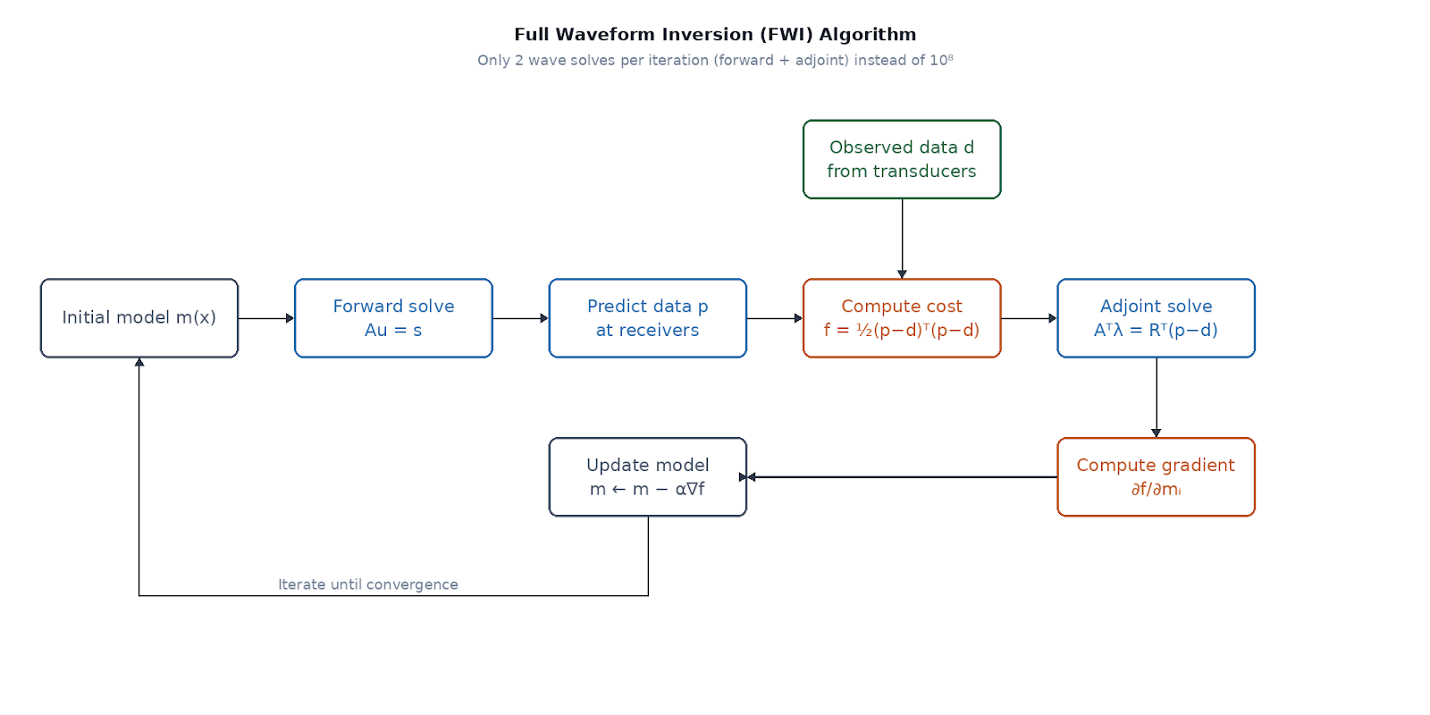
Fig 8. Flowchart of the Full Waveform Inversion algorithm with credits to claude

5. The local curvature in San Francisco

In San Francisco, focused ultrasound has been having a moment since the end of 2024, with the rise of the transcranial focused ultrasound society (tFUS society) and collaborations with local non-profits, including Foresight Institute, Frontier Tower, Stanford University, and the Neurotech at Berkeley. What a time to be alive!

References

[1] Acoustic wave equation. Wikipedia. https://en.wikipedia.org/wiki/Acoustic_wave_equation

[2] Walsh, W. MRI Basics. University of Pennsylvania. https://www.sas.upenn.edu/~wwalsh/MRI%20BASICS.html

[3] MRI coils explanation. YouTube. https://www.youtube.com/watch?v=EMeAC50zjFg

[4] Krug, J. et al. MR-ARFI. Journal of Magnetic Resonance Imaging. https://doi.org/10.1002/jmri.29712

[5] Guasch, L. et al. “Full-waveform inversion imaging of the human brain.” NPJ Digital Medicine, 2020. https://pmc.ncbi.nlm.nih.gov/articles/PMC7060331/

[6] Deffieux, T. et al. Nature Reviews Neurology, 2020. https://www.nature.com/articles/s41582-020-00418-z

[7] Young’s modulus. Wikipedia. https://en.wikipedia.org/wiki/Young%27s_modulus

[8] Guasch, L. et al. Nature Digital Medicine, 2020. https://www.nature.com/articles/s41746-020-0240-8/figures/2